A SynExtend example

Finding COGs and co-localized clusters of COGs with SynExtend

Published

September 23, 2026

Rendering notes

This page is rendered locally and frozen (execute: freeze: auto), so the site build on GitHub does not re-run any code. To re-run it you need:

NCBI EDirect tools (esearch, esummary, xtract) on the PATH seen by R.
The R packages SynExtend (which attaches DECIPHER), DBI, RSQLite, rtracklayer, gggenomes, ggplot2 and tibble.

Libraries

suppressMessages(library(SynExtend))
suppressMessages(library(DBI))
suppressMessages(library(gggenomes))

Warning: package 'gggenomes' was built under R version 4.5.2

Warning: package 'ggplot2' was built under R version 4.5.2

Data collection

Genome assemblies are located with an EDirect query and imported into R with a combination of interacting tools from DECIPHER, rtracklayer, and SynExtend.

# via esearch
# import into R with a combination of
# interacting tools from:
# DECIPHER
# rtracklayer
# and
# SynExtend

EntrezQuery <- paste("esearch -db assembly ",
                     "-query '",
                     "nitrososphaeria[organism] ",
                     'AND "complete genome"[filter] ', # only complete genomes
                     'AND "refseq has annotation"[properties] ', # only genomes with annotations
                     'AND "latest refseq"[filter] ', # only latest
                     'AND "reference genome"[filter] ',
                     "NOT anomalous[filter]' ",
                     '| ',
                     'esummary ',
                     '| ',
                     'xtract -pattern DocumentSummary -element FtpPath_RefSeq',
                     sep = "")

FtPPaths <- system(command = EntrezQuery,
                   intern = TRUE,
                   timeout = 300L) # timeout argument is required for RStudio only

adds <- mapply(SIMPLIFY = TRUE,
               USE.NAMES = FALSE,
               FUN = function(x, y) {
                 paste0(x,
                        "/",
                        y[10],
                        c("_genomic.fna.gz",
                          "_genomic.gff.gz",
                          "_protein.faa.gz"))
               },
               x = FtPPaths,
               y = strsplit(x = FtPPaths,
                            split = "/",
                            fixed = TRUE))
fnas <- adds[1, , drop = TRUE]
gffs <- adds[2, , drop = TRUE]
amns <- adds[3, , drop = TRUE]

tmp01 <- tempfile()
drv <- dbDriver("SQLite")
conn01 <- dbConnect(drv = drv,
                    tmp01)

genecalls <- vector(mode = "list",
                    length = length(fnas))
tmp_con <- file(nullfile(), open = "wt")
pBar <- txtProgressBar(style = 1)
PBAR <- length(fnas)
for (m1 in seq_along(gffs)) {
  Seqs2DB(seqs = fnas[m1],
          dbFile = conn01,
          type = "FASTA",
          identifier = as.character(m1),
          verbose = FALSE)
  # import sends things directly to stderr that are difficult to suppress
  # we can sink those messages and discard them ...
  sink(file = tmp_con,
       type = "message")
  tmp_obj <- rtracklayer::import(con = gffs[m1])
  sink(type = "message")
  genecalls[[m1]] <- SquaregffBy(gff_object = tmp_obj,
                                 verbose = FALSE)
  
  setTxtProgressBar(pb = pBar,
                    value = m1 / PBAR)
}

================================================================================

# close our temp connections
close(tmp_con)
close(pBar)

# genecalls needs names that match the names we gave to our sequences when
# we imported them into the database
names(genecalls) <- seq(length(genecalls))

# this might make finding neighborhoods easier ... ?
all_called_features <- do.call(rbind,
                               genecalls)
all_called_features$source_genome <- rep(as.integer(names(genecalls)),
                                         vapply(X = genecalls,
                                                FUN = function(x) {
                                                  nrow(x)
                                                },
                                                FUN.VALUE = vector(mode = "integer",
                                                                   length = 1)))
id_key <- unlist(lapply(X = seq_along(genecalls),
                        FUN = function(x) {
                          paste(x,
                                genecalls[[x]]$Index,
                                seq(nrow(genecalls[[x]])),
                                sep = "_")
                        }))
all_called_features$id_key <- id_key
rownames(all_called_features) <- NULL

Build a (several) synteny map(s)

Synteny objects are created by the FindSynteny function in the DECIPHER R package. DECIPHER relies heavily on databases, is stable, and mature.

syn <- FindSynteny(dbFile = conn01,
                   verbose = TRUE)

================================================================================

Time difference of 202.45 secs

pairs(syn[1:2, 1:2])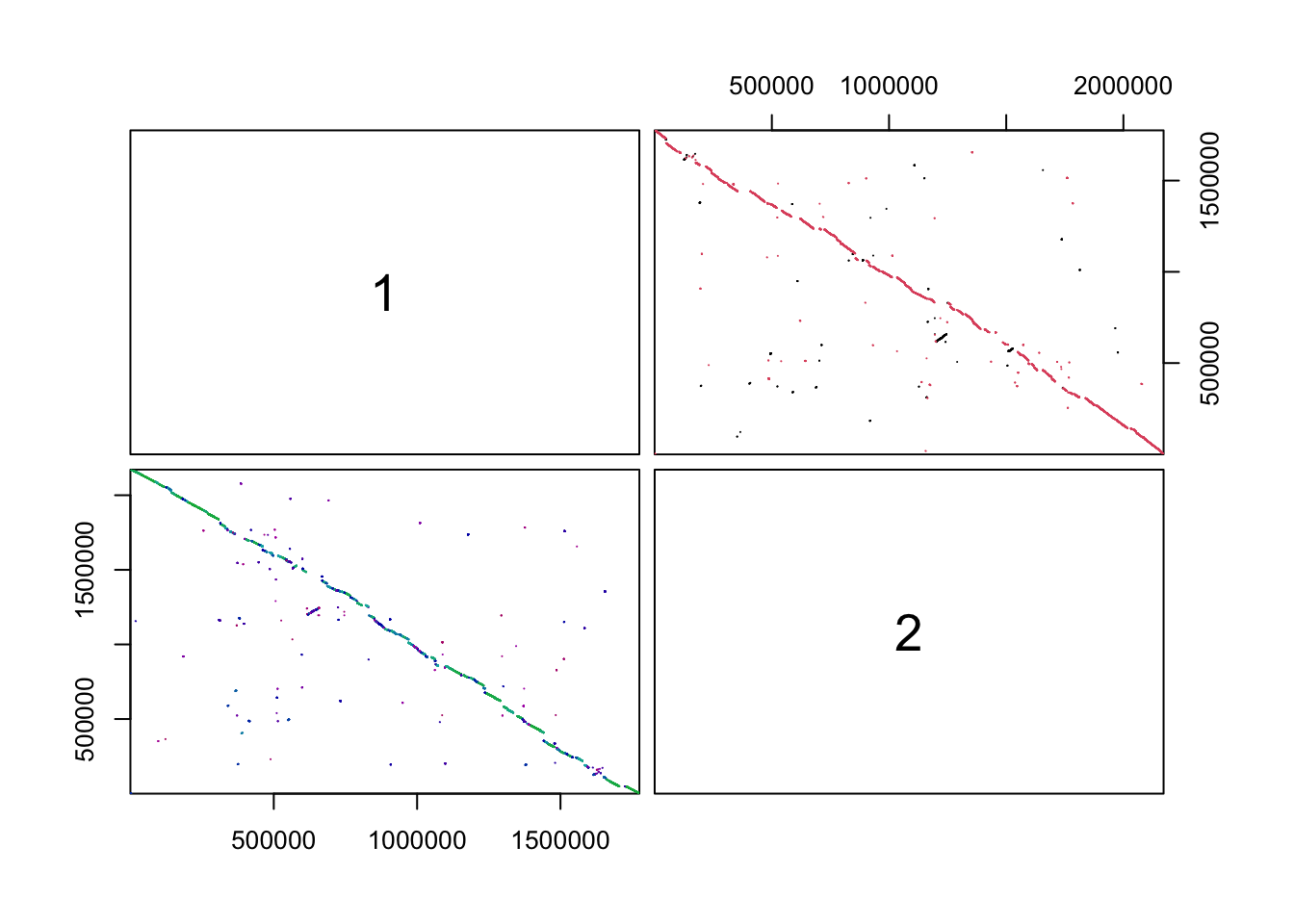

Add context to the maps with gene calls

l01 <- NucleotideOverlap(SyntenyObject = syn,
                         GeneCalls = genecalls,
                         Verbose = TRUE)


Reconciling genecalls.
================================================================================
Finding connected features.
================================================================================
Time difference of 7.428611 secs

Distill the maps into inferred orthologous pairs

p01 <- SummarizePairs(SynExtendObject = l01,
                      DataBase01 = conn01,
                      Verbose = TRUE,
                      Processors = NULL)

Collecting pairs.
================================================================================
Time difference of 59.16772 secs

p02 <- EvaluatePairs(InputPairs = p01,
                     DataBase01 = conn01,
                     Verbose = TRUE)


Generating decoy alignments.

Completed!
Time difference of 1.669005 mins

# close our connection
dbDisconnect(conn01)

Cluster with ExoLabel

Exolabel is a big piece of work that is currently under review and performs out of memory fast label propagation clustering. It is a performant and accessible alternative to clustering methods like MCL.

tmp_pairs <- tempfile()
tmp_out <- tempfile()

write.table(x = p02[, c(1, 2, 13)],
            sep = "\t",
            quote = FALSE,
            append = FALSE,
            col.names = FALSE,
            row.names = FALSE,
            file = tmp_pairs)

ExoLabel(edgelistfiles = tmp_pairs,
         outfile = tmp_out)

$parameters
add_self_loops    attenuation     iterations 
             0              1              5 

$graph_stats
num_vertices    num_edges 
       28066       193162 

$results
[1] "/private/var/folders/xr/t9mzxbj152sd4hhw3pz43q8m0000gn/T/RtmpzAPiCJ/file12a186aa83fa5"

clusts <- read.table(file = tmp_out,
                     header = FALSE)

clusts <- tapply(X = clusts$V1,
                 INDEX = clusts$V2,
                 FUN = c)
# index names are meaningless here
names(clusts) <- NULL

Candidate cluster selection

Keep every single-copy cluster that spans a given set of genomes; in the case of this piece of example code, the entire input set.

# all single copy clusters that span a given set
# in this case, the entire input set

w1 <- lengths(clusts) == length(genecalls)
candidate_clusts <- clusts[w1]

w1 <- vapply(X = candidate_clusts,
             FUN = function(x) {
               ph <- strsplit(x = x,
                              split = "_",
                              fixed = TRUE)
               ph <- vapply(X = ph,
                            FUN = function(x) {
                              x[1]
                            },
                            FUN.VALUE = vector(mode = "character",
                                               length = 1))
               
               if (length(ph) == length(unique(ph))) {
                 return(TRUE)
               } else {
                 return(FALSE)
               }
             },
             FUN.VALUE = vector(mode = "logical",
                                length = 1))
candidate_clusts <- candidate_clusts[w1]

Neighborhood identification

Given a set of candidate clusters, populated with the single-copy features covering the same set of source genomes, return a set identifier.

# given a set of candidate clusters -- populated with the single-copy features
# covering the same set of source genomes -- return some set identifier

target_clusts <- data.frame("cluster_id" = rep(seq_along(candidate_clusts),
                                               lengths(candidate_clusts)),
                            "node" = unlist(candidate_clusts))
w1 <- all_called_features$id_key %in% target_clusts$node
target_features <- all_called_features[w1, ]
w1 <- target_clusts$cluster_id[match(x = target_features$id_key,
                                     table = target_clusts$node)]
target_features$cluster_index <- w1
rownames(target_features) <- NULL

find_neighborhoods() is an ad-hoc helper that returns where neighborhoods are shared across all genomes.

Show the find_neighborhoods() definition

# !!this is an adhoc function and will not scale to sizes that push the bounds
# of R's vector / matrix size limits!!
# strictly return where neighborhoods are shared across genomes, i.e.
# find where a gene_a (genome 1, cluster 1) <--> gene_b (genome 1, cluster 2)
# distance is within max gap AND clusters 1 and 2 similarly have a
# gene_a (genome 2, cluster 1) <--> gene_b (genome 2, cluster 2) within the max
# gap distance in the next genome, and so on
find_neighborhoods <- function(feature_table,
                               max_gap = 5000) {
  
  # we scroll through the upper triangle of the gene table
  l1 <- length(unique(feature_table$source_genome))
  # l2 <- l1 - 1L
  # # genome vs genome search space
  # max_search <- l1 * l2 / 2
  
  # our d1 holding place
  local_neighborhoods <- vector(mode = "list",
                                length = l1)
  # number of ingested clusters
  l3 <- max(feature_table$cluster_index)
  # number of checks
  l4 <- l3 - 1L
  # for list population
  # count <- 1
  for (d1 in seq_len(l1)) {
    # the largest possible neighborhood includes a neighbor from every
    # cluster in the ingested set
    # we're going left to right along the StringSet
    # one direction, and no wrap around ... this technically means we will
    # always miss clusters that span the "start" of the StringSet in circular
    # genomes, but we can live with that for now
    neighborhood_membership <- rep(-1, l3)
    n_idx <- 1
    qt <- feature_table[feature_table$source_genome == d1, ]
    # seq along ingested cluster count minus 1, checking left bound of a
    # to right bound of b
    for (d2 in seq_len(l4)) {
      lp_end <- qt$Stop[d2]
      rp_start <- qt$Start[d2 + 1]
      lp_idx <- qt$Index[d2]
      rp_idx <- qt$Index[d2 + 1]
      if (rp_start - lp_end - 1 <= max_gap &
          lp_idx == rp_idx) {
        neighborhood_membership[c(d2, d2 + 1)] <- n_idx
      } else {
        # skip and increment the index
        n_idx <- n_idx + 1
      }
    }
    neighborhood_membership <- neighborhood_membership[order(qt$cluster_index)]
    local_neighborhoods[[d1]] <- neighborhood_membership
  } # end d1
  neighborhood_matrix <- do.call(rbind,
                                 local_neighborhoods)
  
  # return(neighborhood_matrix)
  
  res <- rep(0, l3)
  for (d1 in seq_len(l4)) {
    for (d2 in (d1 + 1):l3) {
      # this can probably be faster, both in the equality test, and
      # in the search, but this is just example code ...
      # ¯\_(ツ)_/¯
      if (all(neighborhood_matrix[, d1] == neighborhood_matrix[, d2]) &
          all(neighborhood_matrix[, d1] > 0)) {
        if (res[d1] == 0) {
          res[c(d1, d2)] <- d1
        } else {
          res[d2] <- res[d1]
        }
      }
    }
  }
  return(res)
}

# each vector position is either 0 - not in a neighborhood at all
# or > 0, where the integer indicates the neighborhood progenitor in the search
# space, i.e.
# 0, 0, 0, 4, 0, 4
# indicates that clusters 4 and 6 are in a neighborhood
neighboring_clusters <- find_neighborhoods(feature_table = target_features)

Populate neighborhoods around co-occurring sets

populate_neighborhoods() is another ad-hoc helper that pulls every called feature that falls within a flanking window around each co-localized group, in every genome.

Show the populate_neighborhoods() definition

# target_features must be a subset of all_called_features,
# and neighboring_clusters (and the associated id and index) must be 
# from the construction and subsetting, we should assume they're correctly
# sorted, at least for this example
populate_neighborhoods <- function(all_called_features,
                                   target_features,
                                   neighboring_clusters,
                                   flank_bp = 3000,
                                   min_count = 3) {
  
  colocal_vals <- table(neighboring_clusters)
  colocal_ids <- as.integer(names(colocal_vals))
  colocal_sizes <- unname(colocal_vals)
  # drop zero named position if it exists
  # where cluster was not co-localized with any other cluster
  drop_if <- which(colocal_ids == 0)
  if (length(drop_if) > 0) {
    colocal_ids <- colocal_ids[-drop_if]
    colocal_sizes <- colocal_sizes[-drop_if]
  }
  if (length(colocal_ids) < 1 |
      all(colocal_sizes < min_count)) {
    stop("'neighboring_clusters' must imply at least one colocalized group of clusters")
  }
  w1 <- colocal_sizes >= min_count
  colocal_ids <- colocal_ids[w1]
  colocal_sizes <- colocal_sizes[w1]
  if (length(colocal_ids) < 1) {
    stop("'neighboring_clusters' must imply at least one colocalized group of clusters is equal to or greater than 'min_count'")
  }
  
  o1 <- order(colocal_sizes,
              decreasing = TRUE)
  colocal_sizes <- colocal_sizes[o1]
  colocal_ids <- colocal_ids[o1]
  
  # other overhead
  u_genomes <- unique(all_called_features$source_genome)
  
  # for each colocalized group of clusters
  # take the cluster members in each genome, confirm shared contigs, grab
  # their left-est and right-est bounds
  pBar <- txtProgressBar(style = 1)
  PBAR <- length(colocal_ids)
  res <- vector(mode = "list",
                length = PBAR)
  for (d1 in seq_along(colocal_ids)) {
    grouping <- vector(mode = "list",
                       length = length(u_genomes))
    for (d2 in seq_along(u_genomes)) {
      w1 <- which(neighboring_clusters == colocal_ids[d1])
      w1 <- which(target_features$cluster_index %in% w1 &
                    target_features$source_genome == u_genomes[d2])
      # hypothetically this could miss in a different context, but not in the
      # current setup
      current_colocals <- target_features[w1, ]
      
      colocal_left <- min(current_colocals$Start)
      colocal_right <- max(current_colocals$Stop)
      colocal_contig <- unique(current_colocals$Contig)
      
      check_against <- all_called_features[all_called_features$source_genome == u_genomes[d2] &
                                             all_called_features$Contig == colocal_contig, ]
      w2 <- check_against$Start >= (colocal_left - flank_bp)
      w3 <- check_against$Stop <= (colocal_right + flank_bp)
      current_return <- check_against[w2 & w3, ]
      
      # other feature
      current_key <- rep("other", nrow(current_return))
      # clustered feature, but not co-local
      current_key[current_return$id_key %in% target_features$id_key] <- "other shared single-copy"
      # colocalized feature in this window
      current_key[current_return$id_key %in% current_colocals$id_key] <- paste("cluster",
                                                                               current_colocals$cluster_index,
                                                                               sep = "_")
      current_return$other_key <- current_key
      grouping[[d2]] <- current_return
      
    }
    
    res[[d1]] <- do.call(rbind,
                         grouping)
    setTxtProgressBar(pb = pBar,
                      value = d1 / PBAR)
  }
  return(res)
}

populated_neighborhoods <- populate_neighborhoods(all_called_features = all_called_features,
                                                  target_features = target_features,
                                                  neighboring_clusters = neighboring_clusters,
                                                  flank_bp = 3000,
                                                  min_count = 5)

================================================================================

Make the populated neighborhoods ingestible by gggenomes

gggenomes expects a genes data frame, a seqs data frame and a links data frame. We can build these by reconciling all called features, all clustered features, and the co-localization of clusters. We accomplish this with a convert_neighborhood_to_gggenome ad-hoc function.

Show the convert_neighborhood_to_gggenome() definition

# gggenomes expects:
# "genes" df
# "seqs" df
# "links" df
# we need to populate these from the our reconciliation of all called features,
# all clustered features, and the colocalization of clusters

# genome_labels must be a named integer vector with ints representing the
# genome index numbers, and names representing the labels to pass to them
# if they are not supplied, seqs will be named after the contig
# 
# infer the window bounds from the max (stop) and min (start) positions in
# the sets
convert_neighborhood_to_gggenome <- function(neighborhood,
                                             genome_labels = NULL,
                                             dbcrossref_types = c("GenBank",
                                                                  "GeneID")) {
  # loop through the genome indices in the neighborhood DataFrame
  u_genomes <- unique(neighborhood$source_genome)
  if (is.null(genome_labels)) {
    # the current assumption is that we are plotting a single co-localized
    # set per genome, this forces us to one contig per genome, if that preamble
    # changes, this needs to become more sophisticated ...
    genome_labels <- unique(neighborhood$Contig)
  } else {
    genome_labels <- names(genome_labels)[match(x = genome_labels,
                                                table = u_genomes)]
  }
  
  # db cross ref de-mangling, and meaningful-ish feature names
  # if you can cross reference to GeneID, Genbank, or Uniprot, that's
  # pretty nice, but if we can't and have to fall back on the locus assignment
  # we will preference of cross reference used is set by the order of the
  # supplied string
  cr_reconcile <- lapply(X = dbcrossref_types,
                         FUN = function(x) {
                           grepl(pattern = x,
                                 x = neighborhood$Dbxref)
                         })
  cr_hit <- lapply(X = cr_reconcile,
                   FUN = function(x) {
                     any(x)
                   })
  cr_val <- mapply(SIMPLIFY = FALSE,
                   USE.NAMES = FALSE,
                   FUN = function(x, y) {
                     a <- neighborhood$Dbxref[y]
                     a <- gsub(x = a,
                               pattern = paste0(x,
                                                ":"),
                               replacement = "")
                     a <- unlist(a)
                     return(a)
                   },
                   x = dbcrossref_types,
                   y = cr_reconcile)
  
  cr_symbol <- cr_source <- vector(mode = "character",
                                   length = length(neighborhood$Dbxref))
  for (d1 in rev(seq_len(length(dbcrossref_types)))) {
    # we're going in reverse through the crossref type asks, so higher precendence
    # will overwrite
    if (any(cr_hit[[d1]])) {
      cr_symbol[cr_hit[[d1]]] <- cr_val[[d1]]
      cr_source[cr_hit[[d1]]] <- dbcrossref_types[d1]
    }
  }
  if (any(nchar(cr_symbol) == 0)) {
    cr_symbol[nchar(cr_symbol) == 0] <- neighborhood$ID[nchar(cr_symbol) == 0]
    cr_source[nchar(cr_source) == 0] <- "genecall_locus"
  }
  # zero out all the feature bounds against the window left bound
  # if the majority of *co-localized features* are in the negative strand,
  # invert the window
  # capture the window width
  
  w_widths <- vector(mode = "integer",
                     length = length(u_genomes))
  genes <- vector(mode = "list",
                  length = length(u_genomes))
  bin_names <- vector(mode = "list",
                      length = length(u_genomes))
  bin_ids <- bin_length <- vector(mode = "integer",
                                  length = length(u_genomes))
  for (d1 in seq_along(u_genomes)) {
    w1 <- neighborhood$source_genome == u_genomes[d1]
    f_left <- neighborhood$Start[w1]
    f_right <- neighborhood$Stop[w1]
    window_left <- min(f_left)
    windor_right <- max(f_right)
    
    w_widths[d1] <- max(f_right) - min(f_left) + 1
    
    gene_df <- data.frame("seq_id" = as.character(neighborhood$source_genome[w1]),
                          "strand" = neighborhood$Strand[w1],
                          "gene_key" = neighborhood$id_key[w1],
                          "product" = neighborhood$Product[w1],
                          # "type" = neighborhood$Type[w1],
                          "type" = rep("CDS", sum(w1)), # gggenomes thing ...
                          "cr_symbol" = cr_symbol[w1],
                          "cr_source" = cr_source[w1],
                          "start" = f_left - window_left + 1,
                          "end" = f_right - window_left + 1,
                          "group_type" = neighborhood$other_key[w1])
    w2 <- which(gene_df$strand == 1)
    if (length(w2) > 0) {
      ph <- gene_df$start[w2]
      gene_df$start[w2] <- gene_df$end[w2]
      gene_df$end[w2] <- ph
    }
    
    genes[[d1]] <- gene_df
    
    bin_names[d1] <- genome_labels[d1]
    bin_ids[d1] <- u_genomes[d1]
    bin_length[d1] <- w_widths[d1]
  }
  
  # return(list(genome_labels,
  #             u_genomes,
  #             w_widths,
  #             bin_names,
  #             bin_ids,
  #             bin_length))
  # build seqs_df
  seqs_df <- data.frame("bin_id" = genome_labels,
                        "seq_id" = as.character(u_genomes),
                        "length" = w_widths)
  
  links <- vector(mode = "list",
                  length = length(genes) - 1)
  # build links table:
  # id1, start, end, id2, start2, end2
  for (d1 in seq_len(length(genes) - 1)) {
    w1 <- grepl(x = genes[[d1]]$group_type,
                pattern = "^cluster_")
    colocal_subjects <- genes[[d1]]$group_type[w1]
    # in this case we can expect these colocal sets to repeat in every genome
    # that may not always be the case but this function is not written for other
    # use case
    w2 <- which(genes[[d1 + 1]]$group_type %in% colocal_subjects)
    o1 <- match(x = genes[[d1 + 1]]$group_type[w2],
                table = colocal_subjects)
    
    links_df <- data.frame("seq_id" = as.character(genes[[d1]]$seq_id[w1]),
                           "start" = genes[[d1]]$start[w1],
                           "end" = genes[[d1]]$end[w1],
                           "seq_id2" = as.character(genes[[d1 + 1]]$seq_id[w2][o1]),
                           "start2" = genes[[d1 + 1]]$start[w2][o1],
                           "end2" = genes[[d1 + 1]]$end[w2][o1])
    links[[d1]] <- links_df
  }
  links <- do.call(rbind,
                   links)
  
  genes <- do.call(rbind,
                   genes)
  
  res <- list("genes" = genes,
              "seqs" = seqs_df,
              "links" = links)
  return(res)
}

plotting_info <- vector(mode = "list",
                        length = length(populated_neighborhoods))

for (d1 in seq_along(plotting_info)) {
  plotting_info[[d1]] <- convert_neighborhood_to_gggenome(neighborhood = populated_neighborhoods[[d1]])
}

Select and plot a neighborhood

Check the neighborhoods for any that have a large fraction of hypothetical proteins. If none do, just select the first (largest) neighborhood for plotting.

# find a fraction of colocalized seqs that are listed as 'hypothetical'

hyp_frac <- vector(mode = "numeric",
                   length = length(plotting_info))
for (d1 in seq_along(plotting_info)) {
  w1 <- grepl(pattern = "^cluster_",
              x = plotting_info[[d1]]$genes$group_type)
  
  hyp_frac[d1] <- sum(grepl(pattern = "hypothetical",
                            x = plotting_info[[d1]]$genes$product[w1])) / sum(w1)
}

if (any(hyp_frac > 0)) {
  select_neighborhood <- which.max(hyp_frac)
} else {
  select_neighborhood <- 1
}

plot_input <- plotting_info[[select_neighborhood]]

member_groups <- sort(unique(plot_input$genes$group_type[startsWith(plot_input$genes$group_type, "cluster_")]))
fills <- c(stats::setNames(grDevices::hcl.colors(length(member_groups), "Dark 3"),
                           member_groups),
           "other shared single-copy" = "#9ecae1",
           "other" = "grey88")

p <- gggenomes(genes = tibble::as_tibble(plot_input$genes),
               seqs = tibble::as_tibble(plot_input$seqs),
               links = tibble::as_tibble(plot_input$links)) +
  gggenomes::geom_seq() +
  gggenomes::geom_bin_label(expand_left = 0.25) +
  gggenomes::geom_link(fill = "grey80", color = NA) +
  gggenomes::geom_gene(ggplot2::aes(fill = group_type)) +
  ggplot2::scale_fill_manual(values = fills, name = "cluster") +
  ggplot2::labs(title = "Co-localized cluster example") +
  gggenomes::theme_gggenomes_clean()
p
# ggplot2::ggsave("neighborhood_plot.png", p, width = 12, height = 4.5, dpi = 150)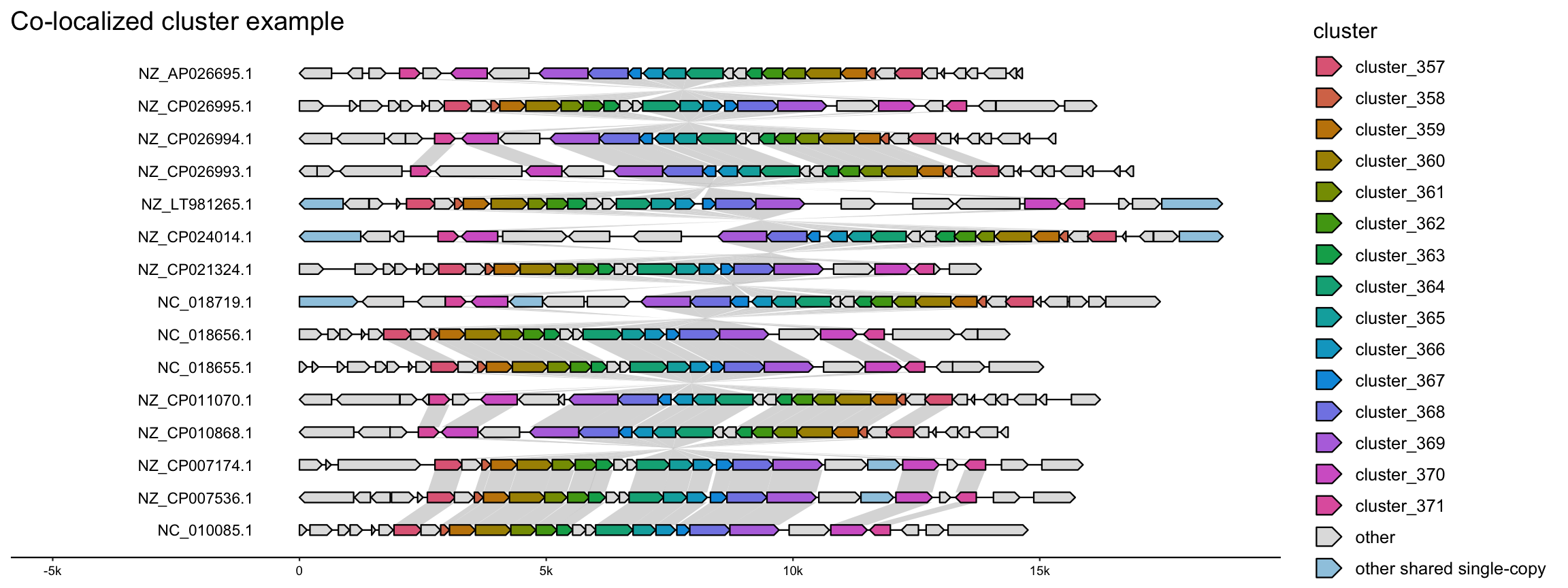

Figure 1: Co-localized single-copy clusters and their flanking features across genomes.

Feature names for the co-localized clusters (from PGAP in this case):

# feature names, from PGAP in this case
w1 <- grepl(x = plot_input$genes$group_type,
            pattern = "^cluster_")
unname(tapply(X = plot_input$genes$product[w1],
              INDEX = plot_input$genes$group_type[w1],
              FUN = function(x) {
                unique(x)
              }))

 [1] "50S ribosomal protein L6"                               
 [2] "30S ribosomal protein S14"                              
 [3] "50S ribosomal protein L5"                               
 [4] "30S ribosomal protein S4e"                              
 [5] "50S ribosomal protein L24"                              
 [6] "50S ribosomal protein L14"                              
 [7] "30S ribosomal protein S17"                              
 [8] "30S ribosomal protein S3"                               
 [9] "50S ribosomal protein L22"                              
[10] "30S ribosomal protein S19"                              
[11] "50S ribosomal protein L23"                              
[12] "50S ribosomal protein L4"                               
[13] "50S ribosomal protein L3"                               
[14] "archaeal proteasome endopeptidase complex subunit alpha"
[15] "DUF371 domain-containing protein"

Session info

sessionInfo()

R version 4.5.1 (2025-06-13)
Platform: aarch64-apple-darwin20
Running under: macOS Sequoia 15.7.9

Matrix products: default
BLAS:   /Library/Frameworks/R.framework/Versions/4.5-arm64/Resources/lib/libRblas.0.dylib 
LAPACK: /Library/Frameworks/R.framework/Versions/4.5-arm64/Resources/lib/libRlapack.dylib;  LAPACK version 3.12.1

locale:
[1] en_US.UTF-8/en_US.UTF-8/en_US.UTF-8/C/en_US.UTF-8/en_US.UTF-8

time zone: America/New_York
tzcode source: internal

attached base packages:
[1] stats4    stats     graphics  grDevices utils     datasets  methods  
[8] base     

other attached packages:
 [1] gggenomes_1.1.3     ggplot2_4.0.1       DBI_1.2.3          
 [4] SynExtend_1.25.2    DECIPHER_3.6.0      Biostrings_2.78.0  
 [7] Seqinfo_1.0.0       XVector_0.50.0      IRanges_2.44.0     
[10] S4Vectors_0.48.0    BiocGenerics_0.56.0 generics_0.1.4     

loaded via a namespace (and not attached):
 [1] SummarizedExperiment_1.40.0 gtable_0.3.6               
 [3] rjson_0.2.23                xfun_0.56                  
 [5] htmlwidgets_1.6.4           lattice_0.22-7             
 [7] Biobase_2.70.0              tzdb_0.5.0                 
 [9] vctrs_0.6.5                 tools_4.5.1                
[11] bitops_1.0-9                curl_7.0.0                 
[13] parallel_4.5.1              tibble_3.3.0               
[15] RSQLite_2.4.5               blob_1.2.4                 
[17] pkgconfig_2.0.3             Matrix_1.7-4               
[19] RColorBrewer_1.1-3          cigarillo_1.0.0            
[21] S7_0.2.1                    lifecycle_1.0.5            
[23] compiler_4.5.1              farver_2.1.2               
[25] stringr_1.6.0               Rsamtools_2.26.0           
[27] codetools_0.2-20            htmltools_0.5.9            
[29] RCurl_1.98-1.17             yaml_2.3.11                
[31] pillar_1.11.1               crayon_1.5.3               
[33] tidyr_1.3.1                 BiocParallel_1.44.0        
[35] DelayedArray_0.36.0         cachem_1.1.0               
[37] abind_1.4-8                 tidyselect_1.2.1           
[39] digest_0.6.39               stringi_1.8.7              
[41] dplyr_1.1.4                 purrr_1.2.0                
[43] restfulr_0.0.16             labeling_0.4.3             
[45] fastmap_1.2.0               grid_4.5.1                 
[47] colorspace_2.1-3            SparseArray_1.10.8         
[49] cli_3.6.6                   magrittr_2.0.4             
[51] S4Arrays_1.10.1             XML_3.99-0.20              
[53] readr_2.2.0                 withr_3.0.2                
[55] scales_1.4.0                bit64_4.6.0-1              
[57] rmarkdown_2.30              httr_1.4.7                 
[59] matrixStats_1.5.0           bit_4.6.0                  
[61] hms_1.1.4                   memoise_2.0.1              
[63] evaluate_1.0.5              knitr_1.50                 
[65] GenomicRanges_1.62.1        BiocIO_1.20.0              
[67] rtracklayer_1.70.0          rlang_1.2.0                
[69] glue_1.8.0                  jsonlite_2.0.0             
[71] R6_2.6.1                    MatrixGenerics_1.22.0      
[73] GenomicAlignments_1.46.0