
Orthology inference with SynExtend - Simple
A simple Pipeline
Introduction
As this is a simple workflow, there’s not much dependencies here. This example code is so simple that it’s probably best suited for users who already have a fairly complex understanding of orthology inference methods and paradigms. The document that this page was knit from can be found in the ’_source’ folder in the associated github repo. Examples targeting multiple use cases, and folks less entrenched in the field will be coming soon!
Libraries
This workflow is very barebones, the only dependency not loaded with SynExtend is RSQLite. There are a few other tools within synextend, and there are many uses for inferred orthologous pairs, so its worth assuming that any complex steps that data generated in pipeline like this gets passed to may require a few more libraries.
suppressMessages(library(SynExtend))
suppressMessages(library(RSQLite))
Data Collection
We’re just pulling a pair of kitasatospora genomes from the NCBI FTP site. Future example will leverage the NCBI’s edirect tools.
ftps <- c("https://ftp.ncbi.nlm.nih.gov/genomes/all/GCF/948/472/415/GCF_948472415.1_JK4103/",
          "https://ftp.ncbi.nlm.nih.gov/genomes/all/GCF/036/010/405/GCF_036010405.1_ASM3601040v1/")

adds <- mapply(SIMPLIFY = TRUE,
               USE.NAMES = FALSE,
               FUN = function(x, y) {
                 paste0(x,
                        "/",
                        y[10],
                        c("_genomic.fna.gz",
                          "_genomic.gff.gz",
                          "_protein.faa.gz"))
               },
               x = ftps,
               y = strsplit(x = ftps,
                            split = "/",
                            fixed = TRUE))
fnas <- adds[1, ]
gffs <- adds[2, ]
amns <- adds[3, ]
Data Processing
The initial data processing for this pipeline involves using DECIPHER to construct a database of the genomic sequences that we’re comparing. We also need to collect the PGAP gene calls for these genomes.
dbpath <- tempfile()
conn01 <- dbConnect(SQLite(), dbpath)
genecalls2 <- vector(mode = "list",
                     length = length(gffs))

for (m1 in seq_along(fnas)) {
  Seqs2DB(seqs = fnas[m1],
          type = "FASTA",
          dbFile = conn01,
          identifier = as.character(m1),
          verbose = TRUE)
  genecalls2[[m1]] <- gffToDataFrame(GFF = gffs[m1],
                                     Verbose = TRUE)
}
## Reading FASTA file chunk 1
##
## 3 total sequences in table Seqs.
## Time difference of 1.23 secs
##
## ================================================================================
## Time difference of 1.213479 mins
## Reading FASTA file chunk 1
##
## Added 1 new sequence to table Seqs.
## 4 total sequences in table Seqs.
## Time difference of 1.31 secs
##
## ================================================================================
## Time difference of 1.481217 mins
names(genecalls2) <- seq(length(genecalls2))
Initial pipeline steps
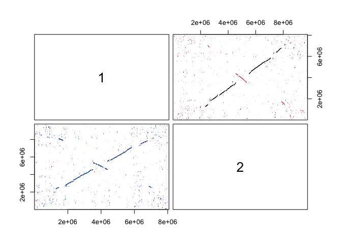
Once all our data is collected, we can start with the construction of a synteny map (with FindSynteny()), followed by overlaying our genecalls on top of that map (with NucleotideOverlap()). Lastly we do a little data munging with PrepareSeqs(), which appends coding and non-coding sequences onto the DECIPHER database for simpler access later.
syn <- FindSynteny(dbFile = conn01,
                   verbose = TRUE)
## ================================================================================
##
## Time difference of 59.29 secs
pairs(syn)
l01 <- NucleotideOverlap(SyntenyObject = syn,
                         GeneCalls = genecalls2,
                         Verbose = TRUE)
##
## Reconciling genecalls.
## ================================================================================
## Finding connected features.
## ================================================================================
## Time difference of 0.4730809 secs
PrepareSeqs(SynExtendObject = l01,
            DataBase01 = conn01,
            Verbose = TRUE)
## Preparing overhead data.
## ================================================================================
## Complete!
## Time difference of 1.663025 secs
Inferrence evaluation steps
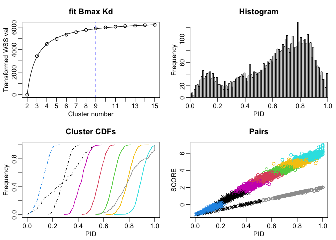
We can take the synteny map, with the overlaid gene calls (which are at this point an attribute to the object l01), and summarize every ‘cell’ in this grid that has a syntenic hit inside it. This gives us a list of candidate ortholog inferences (object p01 in the code below). Following this summarization (which includes alignment and a few other details) we perform a modestly naive k-means clustering step that bins the candidate inferences in to clusters with similar alignment and sequence comparison statistics. At this point, we can drop pairs that belong to comparison communities that appear random, spurious, or below our alignment quality expectations, and we’ll be left with a slightly (depending on the stringency of our thresholds) filtered list pairs. Lastly, we then compete our candidates amongst each other to distill our pairs list into inferred orthologs (one-to-one relationships).
p01 <- SummarizePairs(SynExtendObject = l01,
                      DataBase01 = conn01,
                      Verbose = TRUE,
                      IndexParams = list("K" = 5))
## Collecting pairs.
## ================================================================================
## Time difference of 1.585992 mins
p02 <- ClusterByK(SynExtendObject = p01,
                  Verbose = TRUE,
                  ShowPlot = TRUE)
## ================================================================================
## Time difference of 2.581517 secs
p03 <- CompetePairs(SynExtendObject = p02[p02$ClusterID %in% which(attr(x = p02,
                                                                        which = "Retain")), ],
                    Verbose = TRUE,
                    PollContext = TRUE)
## ================================================================================
## Time difference of 0.567996 secs
Internal competition between pairs can be controlled in a variety of ways, including allowing cross-contig competitions or not, or allowing local syntenic block context to weigh in on these competitions or not. This step is the most recently added so it may change slightly in form or implemention.
Some plots
hist(x = p03$PID,
     breaks = seq(from = 0,
                  by = 0.01,
                  to = 1),
     xaxs = "i",
     yaxs = "i",
     main = "Orthologous pairs with background scores included",
     xlab = "PID")
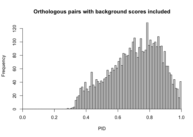
A histogram of PIDs for inferred orthologs! What a user is interested in doing with these pairs is dependent upon their research goals, and further examples will expand on the inner workings of this pipeline, and potential use cases for these pairs lists.
Final thoughts
SynExtend has been a bit of a meandering project so far. Part of the reason for it living in the research doldrums for so long is that there aren’t particularly good methods for benchmarking orthology inference, particularly in the space where this tool is intended for use (large scale prokaryotic genomics). The goal here was to build a backbone of orthology inference that was entirely based within R (with minimal dependencies!) and was relatively quick. SynExtend has been through a lot of itertions at this point, with continually improving inference quality and varying degrees of resource usage improvements, and will likely go through several more before, and after publication.
sessionInfo()
## R version 4.4.2 (2024-10-31)
## Platform: x86_64-apple-darwin20
## Running under: macOS Sonoma 14.3
##
## Matrix products: default
## BLAS:   /Library/Frameworks/R.framework/Versions/4.4-x86_64/Resources/lib/libRblas.0.dylib
## LAPACK: /Library/Frameworks/R.framework/Versions/4.4-x86_64/Resources/lib/libRlapack.dylib;  LAPACK version 3.12.0
##
## locale:
## [1] en_US.UTF-8/en_US.UTF-8/en_US.UTF-8/C/en_US.UTF-8/en_US.UTF-8
##
## time zone: America/New_York
## tzcode source: internal
##
## attached base packages:
## [1] stats4    stats     graphics  grDevices utils     datasets  methods
## [8] base
##
## other attached packages:
##  [1] RSQLite_2.3.9       SynExtend_1.19.7    DECIPHER_3.2.0
##  [4] Biostrings_2.74.0   GenomeInfoDb_1.42.1 XVector_0.46.0
##  [7] IRanges_2.40.1      S4Vectors_0.44.0    BiocGenerics_0.52.0
## [10] knitr_1.49
##
## loaded via a namespace (and not attached):
##  [1] vctrs_0.6.5             crayon_1.5.3            httr_1.4.7
##  [4] cli_3.6.3               rlang_1.1.4             xfun_0.49
##  [7] DBI_1.2.3               UCSC.utils_1.2.0        jsonlite_1.8.9
## [10] bit_4.5.0.1             htmltools_0.5.8.1       rmarkdown_2.29
## [13] evaluate_1.0.1          fastmap_1.2.0           yaml_2.3.10
## [16] memoise_2.0.1           compiler_4.4.2          blob_1.2.4
## [19] pkgconfig_2.0.3         rstudioapi_0.17.1       digest_0.6.37
## [22] R6_2.5.1                parallel_4.4.2          GenomeInfoDbData_1.2.13
## [25] bit64_4.5.2             tools_4.4.2             zlibbioc_1.52.0
## [28] cachem_1.1.0